
You launch a campaign, the landing page traffic looks healthy, and the results still feel off. The headline that “won” may not have won at all, because the sample was too small, the audience split was uneven, or the tracking missed enough visits to blur the outcome. That's the point where sample size calculation stops being a statistics exercise and starts becoming a decision-making tool.
Get it right, and you can defend your numbers in a room full of marketers, analysts, and skeptics. Get it wrong, and you either act on noise or wait too long for a test that never needed that much traffic in the first place. A good planning process also helps you judge measurement quality, which is why teams that care about experiment rigor often pair it with broader analytics effectiveness reviews like measuring marketing effectiveness.
Why Sample Size Calculation Matters
A growth team once ran a headline test on a busy landing page and declared a winner after a short run. The problem wasn't the copy, it was the math behind the decision. The team had enough visits to feel confident, but not enough usable observations to trust the result, so the “winning” headline kept the old conversion pattern when it was rolled out more broadly.
That kind of mistake is expensive because it looks decisive at first glance. A weak sample can make a real lift disappear into randomness, while an oversized sample can keep a decision waiting long after the business already needed an answer. The value of sample size calculation is that it turns a vague sense of “enough data” into a planned threshold you can explain to a stakeholder.
A second reason it matters is that planning and measurement are tied together. If the tracking is flaky, the actual usable sample is smaller than the traffic dashboard suggests. If you want a practical foundation for the measurement side, this explanation of statistical power is a useful companion because it connects the planning question to the risk of false negatives.
For many, the need isn't more theory; it's for a cleaner decision. How much data do we need for this test, this audience, and this level of risk? That's the essential task.
Defining Key Sample Size Metrics
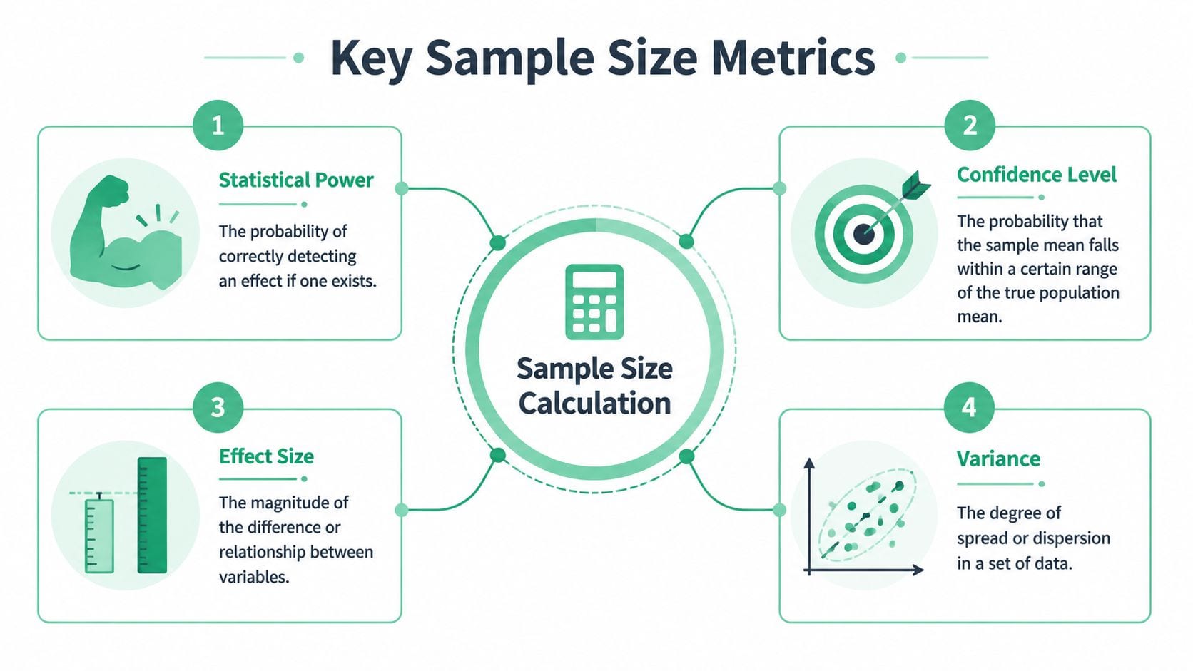
A sample size formula is only as useful as the inputs behind it. In practice, four ideas do most of the work: power, confidence level, effect size, and variance. You can treat them like the four dials on a control panel, because turning one dial usually changes the others, and the sample you need changes with them.
Power and confidence level
Power describes how likely a test is to detect a real change. If power is too low, a real improvement can look like noise, and the team may walk away from a result that mattered. Confidence level sets how strict you want to be before calling a result believable, which is why it reflects the level of caution behind the decision.
A simple planning rule follows from that relationship, more caution usually means a larger sample. A stricter confidence level, or a higher power target, gives you fewer false signals, but it also asks for more data before you can act. That tradeoff is easy to miss if the conversation starts with traffic instead of decision risk.
For a clearer explanation of how statistical power shapes planning, this explanation of statistical power connects the technical idea to the chance of missing a real effect.
Effect size and variance
Effect size is the size of the change you want to detect. That is where many teams get stuck, because prior data are often thin or inconsistent, and the effect you care about may not be obvious. A practical way to handle that uncertainty is to choose a defensible range of plausible effects instead of pretending there is one exact number. For analysts who want a more applied framing, practical effect size insights for analysts is a useful companion.
Practical rule: If prior data are weak, define several reasonable effect sizes, then check how the required sample shifts across that range. Use the range to defend the plan, not a single guess.
That approach is especially helpful when the cost of being wrong is high. In a thin evidence base, a tiny assumed effect can make the sample look unrealistically large, while an inflated assumed effect can make the study look ready before it really is. The defensible middle ground is to test a small set of assumptions and explain why the chosen range fits the business question.
Variance is the other side of the same problem. It describes how spread out the data are, and wide spread means the estimate is less stable. A channel with noisy revenue per user or erratic session value usually needs more observations than a cleaner binary metric, because the calculation has more uncertainty to absorb.
When the data are messy, the planning problem is not only the formula. Tracking gaps can shrink the usable sample after the campaign starts, so teams should plan with attrition in mind rather than assuming every recorded event will survive analysis. That is also why a broader check on measurement quality belongs in the planning stage, and this resource on data-loss prevention is useful background when you are estimating how much clean data you will keep.
Applying Sample Size Formulas for Common Scenarios
A sample size formula only helps when it matches the question in front of you. Estimating a mean is different from estimating a proportion, and comparing two groups adds another layer because the goal shifts from describing a value to detecting a difference between values. The safest way to keep that logic clear is to choose the formula by outcome type first.
| Scenario | Formula | Key Inputs |
|---|---|---|
| Estimate a mean | n = (Z² × σ²) ÷ E² | confidence level, standard deviation, desired precision |
| Estimate a proportion | n = (Z² × p × (1 − p)) ÷ e² | confidence level, expected proportion, margin of error |
| Compare two groups | Use the two-sample comparison formula for the specific test | baseline rate or mean, expected difference, variance, power, confidence level |
For a mean, the main inputs are the standard deviation and the precision you want around the estimate. A wider spread in the data makes the estimate less stable, like trying to measure the level of water in a moving bucket, so you need a larger sample to narrow the uncertainty. This applies to metrics such as average revenue per user, average order value, or time on page.
For a proportion, the question is usually binary, such as conversion or completion. The logic is similar, but the input is a rate instead of a continuous average. If you do not know the true proportion yet, the calculation becomes more conservative because the uncertainty is higher, so it is better to test a few plausible rates than to rely on one weak guess.
For a two-group comparison, the key point is that you are not only estimating a number, you are trying to separate one number from another. That is why A/B tests depend on the baseline level, the size of the difference you want to detect, and the amount of noise in the outcome. If prior data are thin, a defensible approach is to compare several reasonable effect sizes, then choose the one that still makes business sense without pretending the lift is larger than it may be.
Messy digital data usually need another adjustment. Missing tracking, broken events, and late-arriving records can shrink the usable sample after the test starts, so plan for attrition instead of assuming every recorded event will be analyzable. When instrumentation quality is part of the estimate, this overview of A/B test platforms helps show how experimentation tools fit into the planning process.
Useful check: If you cannot say what decision the result will support, the formula will not help much. Start with the business question, then match the math to it.
Worked Examples and Calculators

A formula is easier to trust when you can see it used end to end. The cleanest way to do that is to pick a scenario, write down the assumptions, and then walk through the calculation step by step instead of jumping straight to the result. That's also the right moment to use a calculator, because it lets you test how sensitive the sample is to changes in your assumptions.
A conversion test with a binary outcome
Suppose you're testing a campaign landing page and measuring whether visitors convert or not. You'd start with the current conversion rate, decide what change would matter, and choose the level of certainty you want before shipping a winner. The point isn't to get a fancy number, it's to decide how many usable observations the test needs before the result is believable.
A calculator helps because binary outcomes can feel deceptively simple. A small shift in the expected baseline or the target difference can change the required sample enough to affect scheduling, creative rotation, and budget planning. If you're using an online calculator, check the assumptions before you trust the output, because the calculator only reflects the inputs you give it.
A mean-based revenue experiment
Now consider a test on average revenue per user. The challenge is different because every user can contribute a different amount, and the spread in the data matters as much as the average itself. In those cases, it helps to think about the estimate you're trying to stabilize, not just the test itself.
For hands-on learning, teams often prefer to pair the formula with a walkthrough from a calculator demo. Trackingplan's YouTube channel is a practical place to look for that style of explanation, because seeing the inputs change in real time makes the logic easier to replicate in your own analysis workflow. If your experiment program also depends on reliable implementation and event quality, this platform page can help connect the planning work to the measurement stack.
The main takeaway from the worked examples is simple. Don't treat the calculator as a black box, treat it as a translation layer between your decision and the sample you need.
Handling Real World Data Challenges
Textbook formulas assume the data arrive cleanly, participants stay in the study, and group sizes are what you planned. Digital analytics rarely behaves that neatly. A modern experiment may lose observations to attrition, split traffic unevenly, or collect clustered data across devices, campaigns, or sites.
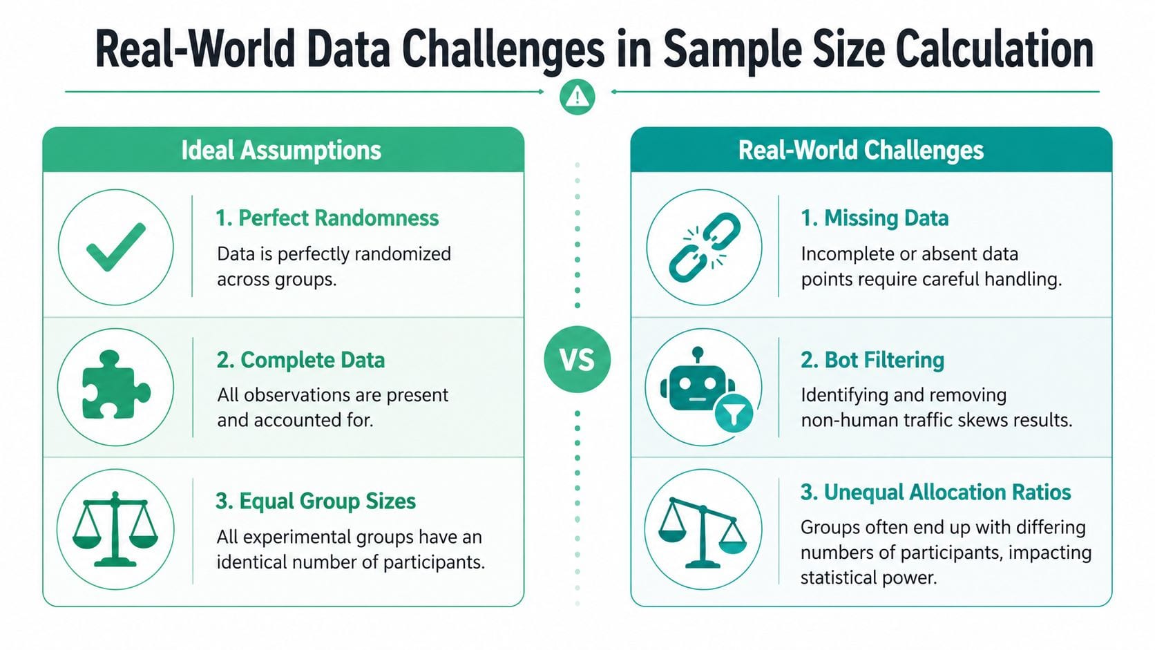
The underlying issue is not just missingness, it's that the realized sample is often smaller or messier than the planned one. Recent sampling guidance says sample size under modern, high-variance, and complex data collection conditions is often undercovered; digital experiments may need inflation rules for attrition, unequal allocation, and clustered sampling (source). That point matters for anyone running experiments through mobile apps, ad platforms, or multi-site workflows.
Where the textbook version breaks
Missing data can turn a good plan into an underpowered test. Bot filtering can reduce the number of valid sessions. Unequal allocation ratios mean one group may need more traffic than the other to deliver the same decision quality. Clustered or stratified sampling can also change the effective amount of information each observation provides.
Practical rule: Plan the sample around usable observations, not raw traffic. If a channel or device tends to create noisy or incomplete records, count that loss before launch.
The same logic applies to peeking at results too early. A midstream look can tempt a team to stop on a noisy bump before the data have stabilized. That's not a sample size problem alone, it's a planning problem, because the stopping rule changes what the data can support.
How teams should inflate the number
The safest approach is to inflate the sample before launch when you expect losses. That buffer should reflect what you've seen in similar campaigns, not wishful thinking. If the workflow is messy, a clean theoretical requirement is rarely enough on its own.
This is also where instrumentation quality and sample size collide. Better tracking won't change the underlying formula, but it can improve the share of observations that are considered valid. For teams that manage multiple tags, pixels, and event streams, this guide to preventing data loss is a sensible complement to the planning side of the problem.
Implications for Analytics Teams and Marketers
A sample size plan only works if the traffic can support it. Marketing budgets limit how much audience you can reach, paid campaigns can change the pace of data collection, and tracking gaps can shrink the pool of usable observations after the fact. That's why the planning question has to include both the experiment design and the measurement setup.
The biggest shift for teams is to stop thinking of sample size as a single number. It's closer to a negotiated target between precision, timeline, and operational reality. If your dashboard is noisy, your confidence in the result should drop. If the tracking is clean and the audience is stable, the same sample may be much more useful.
Teams that work with fast-moving data often use software and AI helpers to manage analysis workflows, and a resource like discover AI tools for data can be useful when you're comparing ways to speed up calculations or reporting. Still, the tool is only as good as the assumptions behind it, so the planning logic has to come first.
Three practical habits help most:
- Buffer the traffic: Plan extra room for unusable sessions, dropouts, or disqualified records before the launch date.
- Clean the instrumentation first: If events or UTM tags are unreliable, fix that before asking the sample to do more work.
- Write down assumptions: Stakeholders trust a sample size recommendation more when they can see what you assumed and why.
That mindset helps marketers, analysts, and agencies make better calls on launch timing and budget allocation. It also keeps the conversation focused on business risk instead of on a calculator output that may not reflect reality.
Conclusion and Next Steps
Good sample size calculation is not about finding the biggest number or the prettiest formula. It's about matching your data plan to the decision in front of you, then making the assumptions explicit enough that someone else can defend them. When prior data are weak, use a range of plausible effect sizes or precision targets instead of pretending the answer is known. When the data collection is messy, inflate for attrition, allocation imbalance, clustering, and any tracking loss you already expect.
A simple checklist keeps the process honest. Define the outcome, choose the right formula, test the assumptions against real traffic, and verify that the tracking can support the planned sample. If the instrumentation is brittle, the math can still be correct while the result remains untrustworthy.
For teams that need repeatable analytics QA, the right next step is to connect planning with ongoing monitoring. That way, your sample size target doesn't fall apart because of broken events, missing parameters, or consent issues that nobody noticed until the dashboard was already wrong. A strong process is what keeps the sample meaningful after launch, not just before it.
Trackingplan helps teams keep analytics clean across web, app, and server-side stacks, so the sample you plan is closer to the sample you analyze. If you're working on experiments, attribution, or campaign reporting, visit Trackingplan to see how automated observability can support more defensible analysis from the first launch onward.